Research-backed calculator guide
Buy vs Rent GPUs for LLM Inference: A Finance-Grade Break-Even
Compare buying and renting GPUs for LLM inference with a transparent break-even model covering utilization, capex, residual value, power, facilities, labor, financing, and capacity risk.
Quick answer
For LLM inference, rent first when demand is uncertain, bursty, geographically distributed, or likely to move to a new GPU generation. Buy can win when you can keep a known configuration productive for years, have the facility and operations capability already in place, and can fund the hardware without making your business fragile. The correct comparison is not a GPU purchase price against a cloud hourly rate. It is the monthly cost of owning divided by productive hours, compared with the fully loaded rental price for the same usable capacity and performance.
A practical break-even formula is:
break-even utilization = monthly owned-GPU cost / (rental price per GPU-hour × available hours per month)
That formula is only meaningful after you define “owned-GPU cost.” Include capital recovery after residual value, financing if the purchase is financed, electricity, cooling, facility or colocation, maintenance, software, support, and a fair share of operations labor. Include the hours the owned system is available, not merely the hours it is doing useful inference. A rented GPU is usually billed by time; AWS, for example, describes On-Demand capacity as hourly or per-second with a 60-second minimum and no long-term commitment.[1]
In the worked example below, an owned H100-class system has an estimated all-in fixed monthly cost of $921.75, while the rental comparison uses a dated Google Cloud list-price observation of $38.32 per hour for an 8-GPU H100 a3-highgpu-8g machine, or $4.79 per GPU-hour before any other charges.[2] Those owned costs are estimates, not a vendor quote, and the cloud number is a published list-price observation rather than a universal quote. Under those assumptions, ownership breaks even at about 26% utilization. Change the power, financing, utilization, GPU generation, or rental contract and the answer changes.
What you are actually comparing
“Buy” can mean several different things. A consumer GPU in an existing workstation is not financially equivalent to an eight-GPU server with NVLink, redundant power, high-speed networking, and a support contract. “Rent” can mean a hyperscaler VM, a specialist GPU cloud, bare metal, a reserved commitment, or interruptible capacity. Compare like with like: model fit, VRAM, quantization, context length, tokens per second, latency target, region, reliability, and data-transfer path.
Start with capacity rather than brand. NVIDIA’s H100 page lists 80 GB of memory for H100 SXM, up to 700 W configurable thermal design power, and 900 GB/s NVLink interconnect.[3] Those specifications matter to an inference budget because a model that does not fit, or a multi-GPU deployment that needs a particular topology, can force you into a different machine class. A cheaper hourly rate is not a saving if it cannot meet the model’s memory or latency requirement.
For ownership, separate cash outlay from economic cost. The cash outlay is what leaves the bank account on purchase day. Economic cost spreads the usable value of the equipment over the period in which it produces service. A simple straight-line capital-recovery estimate is:
monthly capital recovery = (landed capex − expected residual value) / useful life in months
Landed capex should include the GPU, host server, storage, networking, power distribution, installation, and any required rack or colocation setup. Residual value is an assumption. It can be zero, a conservative resale estimate, or a scenario range. Do not treat it as guaranteed cash; resale markets, warranty status, and new GPU generations can change it quickly.
For rental, separate the vendor’s compute quote from add-ons. Google Cloud’s accelerator pricing page explains that GPU-accelerated machines are billed for attached GPUs plus predefined vCPU, memory, and bundled local SSD, and its table displays different hourly, spot, and commitment prices.[2] AWS likewise notes that data transfer, EBS, IP addresses, and other services can create additional charges beyond instance usage.[1] A fair model therefore has a “rental compute” line and separate storage, networking, egress, orchestration, observability, and support lines.
The break-even model
Use one month as the comparison period and make every input explicit.
Owned monthly cost is the sum of monthly capital recovery, financing premium if applicable, electricity and cooling, facility or colocation, maintenance and warranty reserve, software or support, and allocated operations labor. Some of these are fixed while the machine is online. Others vary with runtime. Keep them separate so you can test a scale-to-zero or shutdown policy.
Productive owned hours are available hours multiplied by utilization. If the system is available for 730 hours in a nominal month but only handles useful inference for 40% of that time, it has 292 productive GPU-hours. Queueing, warm-up, failed requests, idle replicas, and headroom for peak traffic should not be silently counted as productive output.
Rental monthly cost is rental hours multiplied by the comparable rate, plus the same non-GPU services needed by the workload. If a rental quote is for a whole machine, divide only after checking how many GPUs are included and whether the workload can use all of them. If throughput differs, normalize by output rather than by GPU-hour:
cost per million output tokens = monthly infrastructure cost / monthly output tokens × 1,000,000
That normalization is important for LLM inference. A GPU that costs twice as much per hour can still be cheaper per million tokens if it produces more than twice the measured throughput at the required latency. Use a benchmark from your model, quantization, prompt mix, batch policy, and context length. Do not substitute a vendor’s theoretical FLOPS for observed tokens per second.
The FinOps Foundation describes FinOps as a practice for business value, timely data-driven decisions, and financial accountability across engineering, finance, and business teams. It also lists taking advantage of the cloud’s variable-cost model as a principle.[4] For this decision, that means tracking utilization and cost by workload, not declaring ownership or rental universally cheaper. A variable rental bill can be valuable when it prevents paying for idle capacity, while a fixed owned asset can be valuable when it is consistently productive.
Worked cost example
This is an illustrative U.S.-dollar scenario checked on 2026-11-02. It is not a quote for a particular buyer.
| Step | Assumption or input | Calculation | Monthly output |
|---|---|---|---|
| 1. Landed owned capex | $17,000 per GPU-equivalent system | GPU, server share, storage, networking and setup estimate | $17,000 upfront |
| 2. Residual value | $3,000 after 36 months | $17,000 − $3,000 | $14,000 depreciable basis |
| 3. Capital recovery | 36-month useful life | $14,000 / 36 | $388.89 |
| 4. Electricity and cooling | 1.0 kW IT load, PUE 1.3, $0.14/kWh | 1.0 × 1.3 × 730 × $0.14 | $132.86 |
| 5. Maintenance reserve | Estimate | Parts, warranty gap and replacement handling | $150.00 |
| 6. Facility and operations allocation | Estimate | Rack/colo share plus routine operator time | $250.00 |
| 7. Owned monthly total | Sum of rows 3–6 | $388.89 + $132.86 + $150 + $250 | $921.75 |
| 8. Rental comparison rate | $38.32/hour for 8 H100s on the cited Google table | $38.32 / 8 GPUs | $4.79/GPU-hour |
At 70% utilization, the owned system produces 511 productive hours in a 730-hour month. Its effective cost is $921.75 / 511 = $1.80 per productive GPU-hour. The comparable rental bill is 511 × $4.79 = $2,448.69 before storage, transfer, and other services. On these assumptions, ownership is lower by about $1,527 per month, but only if the system really achieves that utilization and the estimated facility and operations costs are fair.
At 20% utilization, ownership still costs $921.75 because most of the monthly burden remains. Its effective productive-hour cost rises to $921.75 / 146 = $6.31. Rental compute is 146 × $4.79 = $699.34, so renting is cheaper before considering the value of flexibility. The break-even utilization is $921.75 / ($4.79 × 730) = 26.3%.
The result is sensitive to financing. If the $17,000 purchase is financed, replace straight-line capital recovery with the actual loan payment and fees. At a high interest rate or short repayment period, the owned monthly line increases. The result is also sensitive to the rental comparison: a reserved commitment may reduce the rental rate but add an obligation to consume capacity; spot may reduce the rate but add interruption and restart risk.
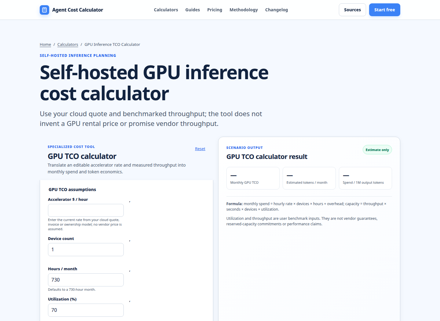
The existing Self-hosted GPU inference cost calculator is useful for testing this kind of scenario. Enter the current quote or ownership-equivalent hourly rate rather than assuming a vendor price, then use measured throughput. The tool’s output should be treated as an estimate, not a performance guarantee.
When renting is usually the safer economic choice
Renting is usually the better starting point when the workload is experimental, seasonal, bursty, or still changing. It preserves cash, lets you test different VRAM sizes and GPU generations, and avoids paying for a machine during a quiet period. It is also useful when users are distributed across regions, when data residency requires several deployment locations, or when capacity must be added quickly for a launch.
Renting also moves some operational burden to the provider, but it does not eliminate it. You still need image management, autoscaling, observability, access control, data transfer planning, and a shutdown policy. A low hourly rate can be overwhelmed by idle instances, attached storage, cross-region traffic, or engineering time spent handling interruptions. For a broader model-cost comparison that keeps units consistent, see Model pricing comparison.
Treat capacity risk as a cost, even when it is not on the invoice. A rental provider may have no capacity in your chosen region or GPU type at the moment you need it. A purchased system gives you more direct control but can fail, require repair, or become obsolete. Keep a second provider or a smaller fallback model in the plan if missing an inference SLO has a business cost.
When buying can win
Buying is more defensible when the model and traffic are stable, utilization is high, the hardware can be kept productive for most of its useful life, and you already have power, cooling, security, networking, and competent operations. It can also be necessary for air-gapped or highly regulated workloads where the available rental options do not satisfy the deployment boundary.
Ownership may improve predictability, but “fixed” does not mean “free.” Include replacement cycles, spare parts, firmware work, security patching, insurance, rack space, energy price changes, and the cost of capital. If a new GPU generation materially improves tokens per dollar, the residual-value assumption may be too optimistic. Model a resale case, a zero-residual case, and a faster refresh case.
A hybrid design is often more realistic than a binary answer. Keep a baseline owned pool for predictable traffic and use rented capacity for peaks, experiments, failover, or model migrations. If the workload includes retrieval, compare the GPU decision with the rest of the pipeline in the RAG, embedding and vector database cost calculator, because embedding, storage, and retrieval costs can change the best architecture.
Run your scenario
Turn this framework into an editable estimate.
Use dated, source-linked assumptions and see cost per request, successful task and month.
A decision checklist for finance and engineering
- Define the service. Record model, quantization, context window, target concurrency, p95 latency, region, and measured tokens per second.
- Price equivalent capacity. Compare the same VRAM, topology, storage, networking, and availability rather than comparing product names.
- Build the owned case. Include landed capex, useful life, residual value, financing, electricity, cooling, facility, maintenance, software, and labor.
- Build the rental case. Include the quote, billing granularity, commitment, spot interruption risk, storage, egress, support, and idle time.
- Run utilization sensitivity. Test at least 20%, 40%, 60%, and 80% productive utilization. Add a peak-headroom case.
- Normalize by output. Compare cost per productive GPU-hour and cost per million output tokens. Use your benchmark, not a theoretical maximum.
- Assign risk. Put a dollar estimate or explicit owner against outage, scarcity, data-transfer, refresh, and procurement risk.
- Review monthly. Actual usage and invoice data should replace estimates. The AI agent development cost estimator can help when GPU spend is only one component of a wider product budget.
FAQ
Is renting a GPU cheaper than buying for LLM inference?
It depends on utilization and the fully loaded owned cost. Renting commonly wins at low or irregular utilization because the bill follows runtime. Buying can win at sustained utilization when capex is spread over enough productive hours and the organization already has facilities and operations. Calculate the break-even utilization instead of applying a universal rule.
What costs are most often missing from a buy-versus-rent comparison?
The common omissions are server and networking components, cooling, rack or colocation, maintenance, operator time, financing, data transfer, storage, idle capacity, and refresh or resale risk. A purchase price alone understates ownership. A GPU hourly quote alone understates rental if the workload also needs persistent storage, egress, monitoring, or support.
Should I compare GPU hours or cost per token?
Use both. GPU-hour is a useful capacity and accounting unit, but LLM inference economics depend on measured throughput and latency. A GPU with higher hourly cost can have a lower cost per million output tokens if it serves more tokens under the same quality and SLO constraints. Benchmark the exact model, quantization, prompt mix, and batching policy.
Does financing change the break-even point?
Yes. Financing replaces or supplements depreciation with actual payment timing and interest. Use the monthly payment, origination fees, required collateral, and any tax or accounting treatment relevant to your organization. If the purchase must be paid upfront, model the value of cash and the runway it consumes even if the accounting expense is spread over several years.
Is a reserved or spot rental comparable to buying?
Only after you price the obligation and risk. A reserved commitment can lower the hourly rate but may charge for unused capacity. Spot can be inexpensive but may interrupt an inference service and require checkpointing or failover. Compare expected productive output, not the lowest advertised number.
How should I handle a mixed owned-and-rented fleet?
Set an owned baseline for the traffic you can forecast, then rent for peaks, experiments, and failover. Track each pool separately and route based on latency, capacity, and marginal cost. Recalculate when traffic shape, model size, or GPU generation changes. A hybrid decision is often more resilient than forcing every request through one procurement model.
Limitations and assumptions
This guide uses an illustrative calculation, not a procurement recommendation or vendor quote. The Google Cloud rate is a dated list-price observation from the cited page and may vary by region, machine type, discounts, commitments, taxes, and additional services. The owned capex, residual value, electricity rate, PUE, maintenance, and operations allocation are scenario estimates. Actual inference throughput depends on model architecture, quantization, batching, context, software stack, and service-level objectives. Recheck published pricing and benchmark the workload before making a purchase or commitment.
Primary sources checked
Pricing and product behavior can change. These sources support the time-sensitive claims in this guide; verify current provider terms before committing spend.