Research-backed calculator guide
DeepInfra Shared API vs Private GPU Deployment: Token-to-GPU Break-Even
Compare DeepInfra shared per-token inference with private GPU deployment using a transparent token-to-GPU break-even worksheet, dated GPU assumptions, and utilization checks.
Quick answer
DeepInfra shared versus private model cost is a comparison between two different meters. A shared endpoint normally turns usage into input-token, cached-input-token, and output-token charges. A private deployment turns capacity into GPU-hours, so the bill continues while the allocated GPU is running even when the request stream is quiet. Do not compare a per-million-token rate with a GPU-hour rate until you add a workload, a measured throughput, and an explicit utilization policy.
For a first-pass decision, calculate both totals for the same month:
shared_cost = input_M × input_rate + cached_input_M × cached_rate + output_M × output_rate
private_cost = GPUs × running_hours × GPU_hour_rate + storage + CPU/RAM + network + operations
The shared option usually has the cleaner economics for unpredictable or low-volume traffic because the meter follows requests. Private capacity can become attractive when a custom checkpoint, isolation boundary, predictable latency, or sustained measured throughput is more important than elasticity. Those are decision conditions, not a promise that either option will be cheaper in every workload.
The example below uses deliberately illustrative shared rates of $0.10 per 1 million input tokens and $0.32 per 1 million output tokens. They are scenario inputs, not a DeepInfra quote. For dated context on the other side of the comparison, the approved provider pages checked on 2026-11-02 list materially different GPU meters: Modal displays per-second GPU prices and says idle resources are not billed [1]; RunPod separates dedicated Pods from Serverless pricing and lists an A100 Pod at $1.79 per hour [2]; Lambda lists A100 and H100 instance rates by GPU-hour while also showing the larger machine configuration around each GPU [3]. Recheck the live contract, region, model, and billing granularity before committing capacity.
What the two DeepInfra choices actually meter
Shared API: pay for the token mix
A shared API estimate needs at least three token buckets. Input tokens are the prompt, system instructions, tools, and retrieved context sent to the model. Cached input tokens are a subset that qualifies for a separate cache rate when the provider and model support it. Output tokens are generated completion or reasoning tokens that the billing record counts as output. If you collapse all three into “total tokens,” you can understate a workload with expensive output or overstate one with a large cacheable prefix.
Write the shared estimate in millions of tokens. For example, 400 million ordinary input tokens at $0.10 per million costs $40. One hundred million output tokens at $0.32 per million costs $32. The shared total is $72 before taxes, gateway fees, retries, or other products. If 200 million of the input tokens are actually cached at $0.02 per million rather than ordinary input, the input line becomes $200M × $0.10 + $200M × $0.02 = $24, reducing the same example to $56. The cache assumption must be measured from usage records, not inferred from a stable-looking prompt.
A shared bill is also sensitive to service tier, rate changes, model changes, and retries. Keep the model identifier and checked date beside every rate. If the application changes from an input-heavy summarizer to an output-heavy agent, the same request count can produce a very different bill. The AI token cost calculator is useful for separating those token classes before you compare deployment modes.
Private deployment: pay for capacity exposure
A private endpoint needs a GPU fit and a running-hours policy. The GPU count is not automatically one: model weights, KV cache, batching target, quantization choice, and high-availability policy can require two or more GPUs. Running hours are the hours each GPU is allocated, not only the seconds during which a user request is being generated. A deployment with two GPUs that stays warm for a 720-hour month has 1,440 GPU-hours.
The simplest private compute line is:
private_GPU_cost = GPU_count × running_hours × GPU_hour_rate
Modal's current page makes the unit conversion visible: its listed H100 SXM rate is $0.001097 per second, which is about $0.001097 × 3,600 = $3.95 per GPU-hour; its A100 80 GB rate of $0.000694 per second is about $2.50 per GPU-hour [1]. RunPod's page, updated October 28, 2026, lists an A100 Pod at $1.79 per hour and a separate A100 Serverless line at $2.72 per hour [2]. Lambda's self-serve table lists A100 SXM at $2.79 per GPU-hour and H100 SXM at $3.99 per GPU-hour for one of the displayed configurations [3]. These are provider-specific observations, not interchangeable quotes for a DeepInfra deployment.
Private economics can improve with scale-to-zero, but scale-to-zero changes the service behavior and does not erase model loading, startup, storage, or control-plane costs. Model three policies separately: always warm, scheduled warm, and scale-to-zero. If your private contract bills only while an instance runs, use observed running hours. If it charges a minimum duration or keeps a replica allocated, use the actual billable unit.
Worked cost example
This U.S.-dollar example is checked on 2026-11-02. It is a transparent scenario, not a vendor invoice. The shared token rates are illustrative inputs chosen to make the arithmetic inspectable. The private A100 rate uses the dated RunPod Pod observation cited above only as an external GPU-hour reference; substitute the current DeepInfra private rate when you have it.
Assume 400 million ordinary input tokens, 100 million output tokens, no cached-input discount, and a private deployment that needs two GPUs. Assume measured private throughput of 18,000 total tokens per second across those two GPUs. The throughput is a workload benchmark assumption, not a theoretical specification. The always-warm case uses 720 running hours per GPU per month. The scale-to-zero case runs only for the measured inference seconds and excludes storage, startup, and control-plane charges so those exclusions remain visible.
| Step | Input or assumption | Calculation | Modeled output |
|---|---|---|---|
| 1. Shared input | 400M input tokens at $0.10/M | 400 × $0.10 | $40.00 |
| 2. Shared output | 100M output tokens at $0.32/M | 100 × $0.32 | $32.00 |
| 3. Shared monthly total | 500M total tokens | $40 + $32 | $72.00 |
| 4. Private always-warm floor | 2 GPUs, 720 hours, $1.79/GPU-hour | 2 × 720 × $1.79 | $2,577.60 |
| 5. Private scale-to-zero compute | 500M tokens at 18,000 tokens/second | 500,000,000 ÷ 18,000 ÷ 3,600 | 7.72 hours elapsed |
| 6. Private scale-to-zero GPU time | Two GPUs for 7.72 hours | 2 × 7.72 × $1.79 | $27.62 |
| 7. Always-warm token break-even | $2,577.60 divided by $0.144/M blended shared rate | $2,577.60 ÷ $0.144 | 17,900M tokens |
The shared blended rate in the last row is based on the scenario mix: (0.8 × $0.10) + (0.2 × $0.32) = $0.144 per million tokens. At 500 million tokens, the always-warm private floor is far above the modeled shared bill. Under these assumptions, the private option would need roughly 17.9 billion similarly mixed tokens per month before its fixed GPU floor equaled the shared token spend. That is a break-even for the cost model, not proof that the private deployment can serve that volume at the required latency.
The scale-to-zero line reverses the raw compute result: $27.62 is below $72. But it is not an apples-to-apples production comparison yet. Add model startup, weight loading, storage, queueing, retries, minimum billing, observability, and the cost of keeping a second replica ready if the service has an availability target. A private deployment can therefore be cheaper on active GPU seconds and still be the worse product choice for interactive traffic.
The throughput threshold is also easy to inspect. With two GPUs at $1.79 per hour and a blended shared rate of $0.144 per million tokens, private active compute costs less than the shared meter when measured aggregate throughput is above approximately:
(2 × $1.79 × 1,000,000) ÷ ($0.144 × 3,600) = 6,906 total tokens/second
That threshold applies only to the active-compute case. It does not include an always-warm floor. It also treats input and output tokens as one blended unit, which is acceptable for a rough screen but not for a final capacity decision. A production worksheet should measure prompt processing and generation separately when the serving stack exposes them.
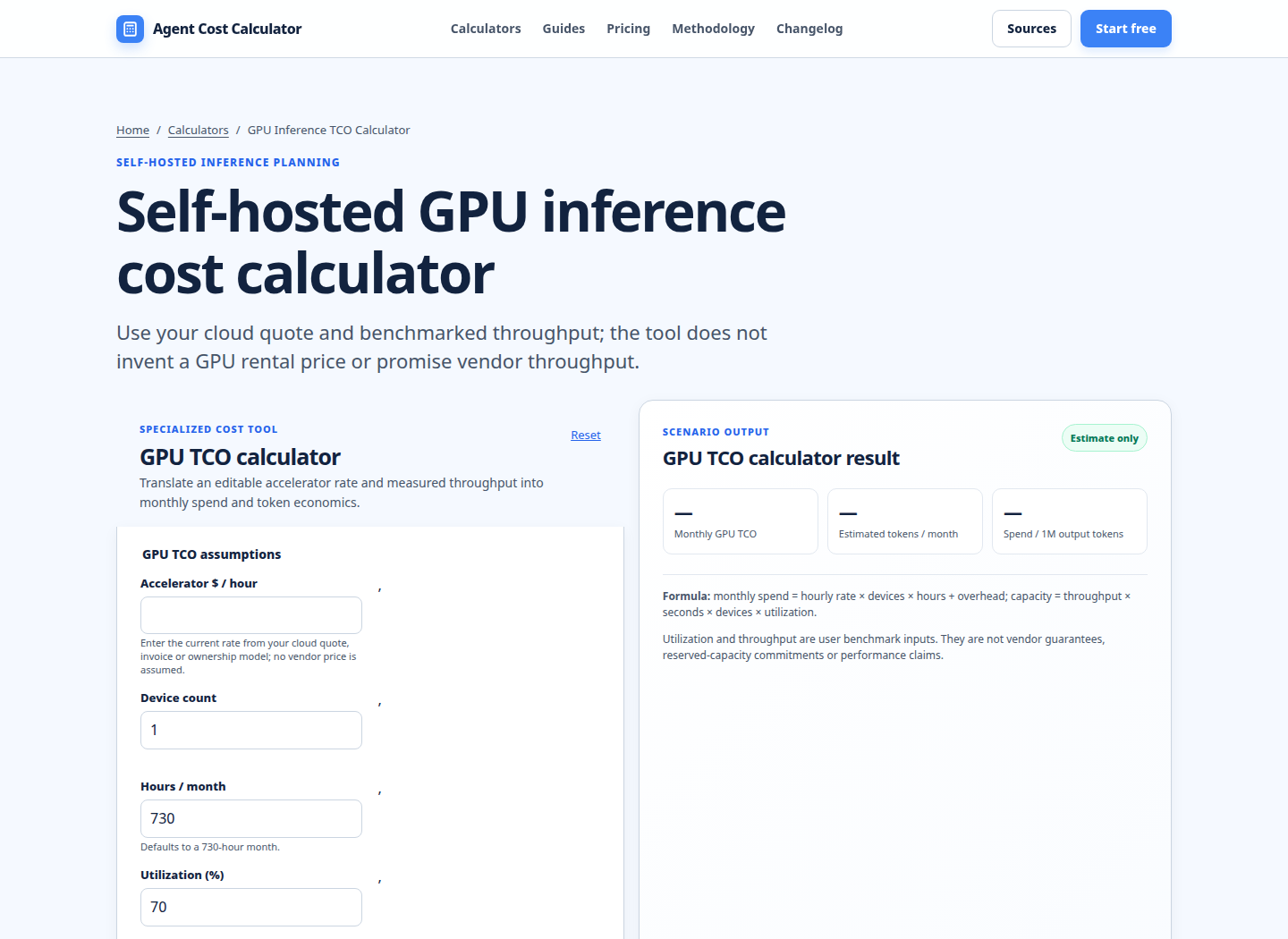
The existing Model pricing comparison helps compare token quotes, while the screenshot’s GPU-oriented fields show the other side of the normalization. Enter one scenario at a time, record the model, GPU count, hours, utilization, and token output, then keep the result with the dated source and benchmark trace. Do not treat a calculator result as a throughput guarantee.
How to find the real break-even for your workload
Start with a 30-day usage export. Sum ordinary input, cached input, and output tokens by model. Keep retries and failed attempts visible rather than silently netting them out. If a request can be routed to multiple models, split the buckets before calculating a blended rate. The AI API invoice reconciliation calculator can help you compare the modeled token totals with the provider invoice once the deployment is live.
Next, benchmark the private candidate with production-shaped prompts. Record tokens per second, time to first token, concurrency, context length, batch size, quantization, and the number of GPUs. A single short prompt at batch size one does not establish the throughput of a long-context agent. Measure at least a quiet case, normal traffic, and a burst. Use p95 or p99 latency if the decision is user-facing.
Then run three private policies. For always warm, multiply every required GPU by every billable hour. For scheduled warm, multiply by the measured daily window and include outside-window cold starts. For scale-to-zero, multiply actual running GPU time by the rate and add startup and retry lines. Compare all three with the shared token total, not with the shared rate alone.
Finally, normalize by the output that matters. For a batch labeling job, cost per million processed tokens may be enough. For an interactive agent, use cost per successful or latency-compliant request. For a fine-tuned model, add the cost of serving the checkpoint and the operational value of isolation. A private deployment may win on control or compliance even when the raw shared bill is lower; that should be stated as a requirement, not disguised as a price saving.
Run your scenario
Turn this framework into an editable estimate.
Use dated, source-linked assumptions and see cost per request, successful task and month.
When shared inference is usually the better starting point
Shared access is a sensible first candidate when demand is spiky, the model is already available, traffic is below the private capacity floor, or the team does not want to operate a serving stack. It also preserves the option to change models without moving weights, tuning batching, or maintaining a dedicated GPU. A shared endpoint can be a poor fit when data isolation, custom weights, deterministic capacity, or a hard latency SLO is non-negotiable.
Watch the failure modes. A low per-token rate does not include your application retries, prompt expansion, tool calls, retrieval, or human review. A high cached-input ratio may disappear after a prompt-template change. A service tier or queue policy can also change the effective latency. Record those lines beside token cost instead of calling the cheapest published rate the total cost.
When private deployment can justify the GPU floor
Private capacity is easier to justify when a checkpoint is not offered as a shared model, when data must stay on dedicated infrastructure, when the model needs custom weights or serving parameters, or when steady traffic keeps the GPU productively occupied. The financial case strengthens when a private GPU can serve multiple internal workloads and the allocation is shared by measured usage rather than charged to one route.
The case weakens when the model needs several GPUs but the traffic is intermittent, when the endpoint must be replicated across regions, or when an operator must keep spare capacity for failover. Include storage, CPU and RAM, network egress, logging, security review, deployment engineering, and shutdown controls. Modal's pricing page, for example, separates GPU, CPU, memory, volume, and network lines rather than presenting GPU compute as the entire bill [1]. RunPod similarly separates Pods, Serverless, Clusters, and storage on its pricing page [2]. Lambda's page shows why a GPU-hour is not always a whole-system comparison: the displayed instance includes vCPU, RAM, and storage alongside the accelerator [3].
FAQ
Is DeepInfra shared API pricing always cheaper than a private GPU?
No. Shared pricing often wins at low or irregular utilization because it avoids an idle-capacity floor, but a measured private deployment can win when it runs at high sustained throughput or is required for custom weights and isolation. Calculate both with the same token mix, GPU count, running-hours policy, and latency target.
How do I compare DeepInfra per-token versus GPU-hour cost?
First calculate the shared bill from ordinary input, cached input, and output tokens. Then calculate private GPU-hours from GPU count, billable running hours, and the current GPU-hour rate. Convert the private result to cost per million tokens only after benchmarking the exact model, prompts, quantization, batching, and concurrency. A GPU-hour quote without throughput is not a token price.
Does cached input change the break-even?
Yes. Cached input can lower the shared side substantially when the repeated prefix qualifies for the provider’s cache meter. Model ordinary and cached input as separate rows and use the observed cache-hit share. If the cache hit rate is uncertain, run low, base, and high cases rather than applying the best discount to every prompt token.
Should a private deployment run 24/7?
Only if the latency, availability, or operational policy justifies the warm floor. Run an always-warm, scheduled-warm, and scale-to-zero case separately. A 24/7 two-GPU deployment at $1.79 per GPU-hour costs $2,577.60 per 720-hour month before storage and other services, even if traffic is quiet for most of the day.
What is the most important private-deployment input?
Measured throughput under the real prompt and latency distribution is usually more useful than a theoretical FLOPS number. It determines how many GPU-hours the workload needs and whether active compute can beat a token meter. Also verify model fit, GPU count, context length, batching, quantization, and the spare capacity required for incidents.
Which costs are excluded from the worked example?
The example excludes taxes, storage, CPU and RAM, network egress, logging, monitoring, gateway fees, deployment labor, model-loading time, retries, failed requests, reserved capacity, regional premiums, and redundancy. It also excludes the business cost of latency misses and data-isolation requirements. Add each line when it is material, and replace all illustrative assumptions with observed invoice and benchmark data.
Limitations and assumptions
This guide is a decision worksheet, not a DeepInfra price guarantee. The shared rates are illustrative scenario inputs. The GPU observations are dated public list prices from the cited pages checked on 2026-11-02; they can change by GPU type, region, plan, taxes, discounts, supply, commitment, and billing granularity. The RunPod A100 Pod rate is not a quote for a DeepInfra private deployment. Use the current contract or account pricing for the final calculation.
The break-even math assumes one consistent token mix and treats active private throughput as a blended token rate. Real inference has different prompt-processing and generation behavior, and a model may need multiple GPUs for memory or latency rather than throughput alone. It also assumes the measured workload is repeatable. Validate with representative prompts, p50/p95 latency, concurrency, error rate, queue time, and at least one burst trace.
For a broader monthly model budget, connect this result to the LLM cost calculator. Keep the shared API estimate, private infrastructure estimate, and non-cost requirements as separate decision columns. That makes a later model change, GPU price change, or utilization change auditable instead of forcing a new comparison from memory.
Primary sources checked
Pricing and product behavior can change. These sources support the time-sensitive claims in this guide; verify current provider terms before committing spend.